Pixel Deflection - a simple transformation based defense
Change local pixel arrangement and then denoise using wavelet transform
Paper: arXiv Code: GitHub Jupyter Notebook: Source
What
- Select a random pixel and replace it with another randomly selected pixel from a local neighborhood; we call this as pixel deflection (PD).
- Use a class-activation type map (R-CAM) to select the pixel to deflect. The less important the pixel for classification, the higher the chances that it will get deflected.
- Do a soft shrinkage over the wavelet domain to remove the added noise (WD).
Why
- PD changes local statistics without affecting the global statistics. Adversarial examples rely on specific activations; PD changes that but not enough to change the overall image category.
- Most attacks are agnostic to the presence of semantic objects in the image; by picking more pixels outside the regions-of-interest we increase the likelihood of destroying the adversarial perturbation but not much of the content.
- Classifiers are trained on images without such (PD) noise. We can smooth the impact of such noise by denoising, for which we found out that BayesShrink on DWT works best.
Table of Contents
Load the requirements
import numpy as np
%matplotlib inline
import matplotlib.pyplot as plt
from random import randint, uniform
Load the classifier
Classifier can be easily changed to inception_v3, vgg19, xception, etc see this
from keras.preprocessing import image
from keras.applications.resnet50 import ResNet50, preprocess_input, decode_predictions
model = ResNet50(weights='imagenet')
def load_image(img_path):
    img = image.load_img(img_path, target_size=(224,224))
    img = image.img_to_array(img)
    true_label = img_path.split('/')[-1].split('_')[0]
    return img, true_label
def visualize_classification(class_names, probs, image, true_class=-1):
    fig, (ax1, ax2) = plt.subplots(1, 2, figsize=(12, 6))
    fig.sca(ax1)

    ax1.imshow(image.astype('uint8'))
    ax1.set_xticks([])
    ax1.set_yticks([])
    ax1.set_title('Image')

    y_pos = np.arange(len(class_names))
    barlist = ax2.bar(y_pos, probs, align='center', alpha=0.5)
    if true_class >= 0 and true_class <= 4:
        barlist[true_class].set_color('g')
    ax2.set_xticks(y_pos, minor=False)
    ax2.set_xticklabels(class_names, minor=False, rotation='vertical')
    ax2.set_ylabel('Probability of given class')
    ax2.set_title('Classification')

    for bar in barlist:
        v = bar.get_height()
        ax2.text(bar.get_x() + bar.get_width()/2., 1.02*v, '%.2f' % v, ha='center')
This classification function works for multiple images in a batch. However, visualization is limited to the first image in the batch. See our GitHub code for better batch processing functions.
def classify_images(images_arr, true_label, visualize=False):
    images = preprocess_input(np.stack(images_arr,axis=0))
    predictions = decode_predictions(model.predict(images),top=5)
    labels, class_names, probs = [], [], []
    for p in predictions:
        labels.append([i[0] for i in p])
        class_names.append([i[1] for i in p])
        probs.append([i[2] for i in p])

    if visualize:
        label_index = labels[0].index(true_label) if true_label in labels[0] else -1
        visualize_classification(class_names[0], probs[0], images_arr[0], label_index)

    return labels, class_names, probs
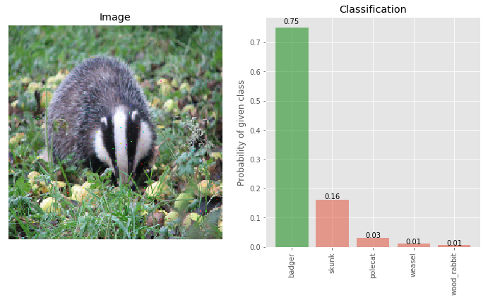
Load and classify the original image
img_clean, true_label = load_image('originals/n02447366_00008562.png')
_ = classify_images([img_clean], true_label, visualize=True)
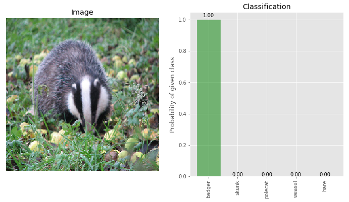
Green color bar indicates the ‘true’ class of the image. The image is correctly classified as ‘badger’ with 100% confidence.
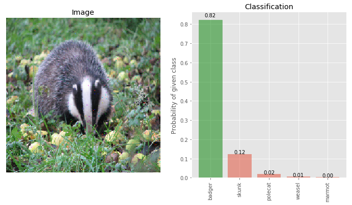
Load and classify the adversarial image
img_adversary, true_label = load_image('images/n02447366_00008562.png')
_ = classify_images([img_adversary], true_label, visualize=True)
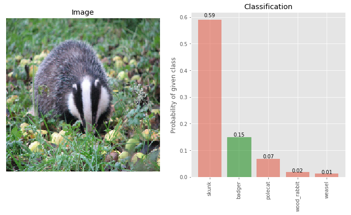
The true class ‘badger’ is now only 15% and ‘skunk’ is the most likely class with 59% classification. This adversary was obtained using IGSM attack model. See this for the attack code.
Pixel Deflection
In our paper, we use pixel deflection with a activation map, but first let’s look at pixel deflection without any maps.
def pixel_deflection_without_map(img, deflections, window):
    img = np.copy(img)
    H, W, C = img.shape
    while deflections > 0:
        #for consistency, when we deflect the given pixel from all the three channels.
        for c in range(C):
            x,y = randint(0,H-1), randint(0,W-1)
            while True: #this is to ensure that PD pixel lies inside the image
                a,b = randint(-1*window,window), randint(-1*window,window)
                if x+a < H and x+a > 0 and y+b < W and y+b > 0: break
            # calling pixel deflection as pixel swap would be a misnomer,
            # as we can see below, it is one way copy
            img[x,y,c] = img[x+a,y+b,c]
        deflections -= 1
    return img
# pixel deflection on adversarial image
img_deflected = pixel_deflection_without_map(img_adversary, deflections=200, window=10)
_ = classify_images([img_deflected], true_label, visualize=True)
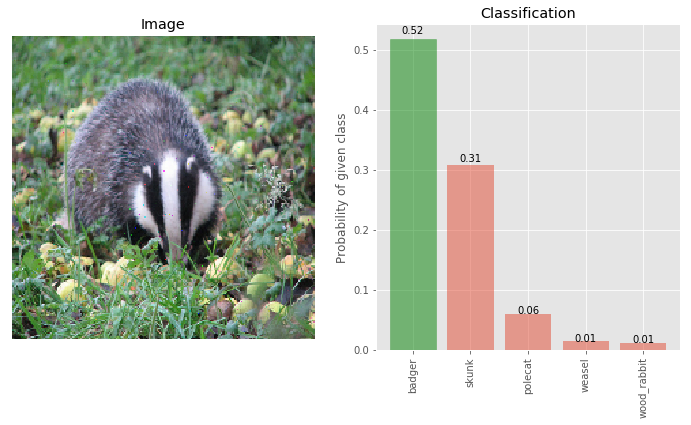
Pixel Deflection is able to retrieve the original class of the image, although the confidence of the true class badger has gone down significantly when compared with the clean image - from 99.7% to 52%.
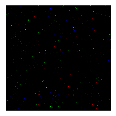
Let’s see the pixels that were deflected.
# deflected pixels
diff = img_adversary - img_deflected
plt.imshow(diff.astype('uint8'))
_=plt.xticks([]), plt.yticks([])
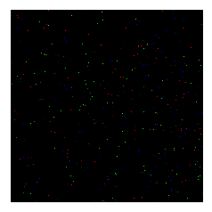
Since we are not using any map, the probability of selecting any pixel in the image is equally likely. If deflecting 200 pixels can cause such a big change in the class probabilities (skunk from 59% from 25% and badger from 15% to 54%) then it begs the question, how much impact will this transformation (pixel deflection) have on the clean images.
Impact on the clean image
For most transformation-based defenses impact on the clean image is too severe, which makes them less useful (e.g. JPEG, TVM) However, the impact of Pixel Deflection on the clean image is almost negligible.
# deflections on clean image
img_clean_deflected = pixel_deflection_without_map(img_clean, deflections=200, window=10)
_ = classify_images([img_clean_deflected], true_label, visualize=True)

The probability of the true class being badger remains at 100%. Let’s investigate the diff with the clean image to see if the image was really transformed.
diff = img_clean - img_clean_deflected
plt.imshow(diff.astype('uint8'))
_=plt.xticks([]), plt.yticks([])
Impact of increasing number of deflections
Increasing the number of deflections significantly increases the accuracy of the recovery of the true class.
# More deflections on adversarial image
img_deflected_more = pixel_deflection_without_map(img_adversary, deflections=600, window=10)
_ = classify_images([img_deflected_more], true_label, visualize=True)
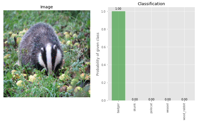
Now the accuracy jumps to 75% but it does not degrade the accuracy on the clean image, as shown below.
# More deflections on clean image
img_clean_deflected_more = pixel_deflection_without_map(img_clean, deflections=600, window=10)
_ = classify_images([img_clean_deflected_more], true_label, visualize=True)
Results so far
| Class | Clean | Adversary | Pixel Deflection |
|---|---|---|---|
| True class - Badger | 100 | 15 | 75 |
| Adversary - Skunk | 0.0 | 59 | 16 |
Wavelet Denoiser
As we state in our paper, pixel-deflection is a form of artificial noise, and denoising this image will get rid of some of this noise. Let’s see what happens after applying wavelet denoising.
from skimage.restoration import denoise_wavelet
def denoiser(img):
    return denoise_wavelet(img/255.0, sigma=0.04, mode='soft', multichannel=True, convert2ycbcr=True, method='BayesShrink')*255.0
Here we show results only for wavelet denoising, the best of several methods. In our paper, we have reported results for various other forms of denoising. To experiment with other types of denoising see this
img_deflected_denoised = denoiser(img_deflected)
_ = classify_images([img_deflected_denoised], true_label, visualize=True)
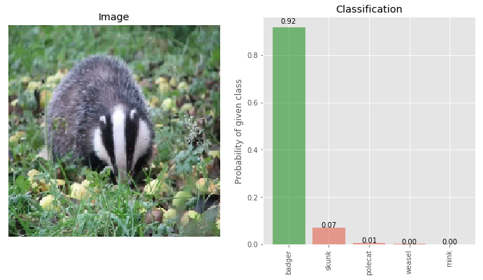
We can see that the confidence on the true class being badger has gone up from 52 to 92 and the adversary class confidence has gone down from 25 to 7. Thus, when we combine Pixel Deflection and Wavelet Denoising, the overall effect is —-
| Class | Clean | Adversary | PD + WD |
|---|---|---|---|
| True class - Badger | 100 | 15 | 92 |
| Adversary - Skunk | 0.0 | 59 | 07 |
Attacks are non-localized
In our paper, we analyzed the location of pixels where the adversary adds the perturbation and found out that most attacks are agnostic to the presence of semantic objects. The correlation between pixels of class-object and pixels perturbed by attacks is very low. Shown below is the average location of adversarial perturbation for some of the major known attacks.

The top left image shows the average location of the object (corresponding to the true class of the image) on a clean image. It is no surprise that most objects of interest are in the center of the image. This could just be human bias for taking pictures especially those which are part of ImageNet.
We take advantage of the a non-localized adversary by deflecting more pixels that are outside the regions-of-interest for a given image. Since precise boundaries are not needed, it is sufficient to obtain a weak localization technique like Class Activation Map. However, we found out that CAM has an inherent weakness when it comes to adversarial images.
CAM vs Robust Activation Maps
Class Activation Maps are heatmaps which highlight the areas most discriminative for a given image and a given class. This works well when the image contains the object given as the class but not so much if the given class has no presence in the image. In a given adversarial image by definition, the ‘class’ of the image is not the same as the true class. Thus, generating CAMs for dversarial images is difficult.
In order to overcome this, we propose a robust version of CAM. If we see the Top-5 predictions for the adversarial image img_adversary other than the ‘adversarial class’, it is no surprise that most of these classes are closely related to the true class even if not the same; skunk, polecat, weasel, and mink are all similar looking animals. This is a well-known side effect of ImageNet because a thousand classes of ImageNet have a lot of fine-grained classes of similar objects/species.
Robust Activation Map is geometric mean of CAM obtained using the top-K classes. By taking the top-K classes, we average out the impact that a single bad adversarial class may have on the activation map.
For more details on robust CAMs we refer the reader to our paper.
Here is a visual comparison of CAM and robust version of CAM.

Apply R-CAM
from scipy.misc import imread
from matplotlib.colors import Normalize

# We normalize the map, because rcam_prob is treated
# as probability values
rcam_prob = Normalize()(imread('maps/n02447366_00008562.png'))

f, ax = plt.subplots(1,3, figsize=(18, 6))
ax[0].imshow(img_clean.astype('uint8'))
ax[0].set_title('Original Image')
ax[1].imshow(rcam_prob)
ax[1].set_title('Robust CAM')
ax[2].imshow(rcam_prob, cmap='jet', alpha=0.6)
ax[2].imshow(img_clean.astype('uint8'), alpha=0.4)
ax[2].set_title('Overlayed')
for ax_ in ax:
    ax_.set_xticks([])
    ax_.set_yticks([])
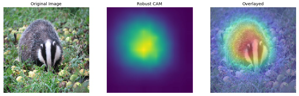
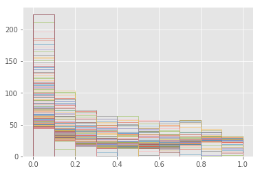
Show below is the distribution of the RCAM probabilities. Significant portion of the image has low value regions; pixels from these regions are most likely to be deflected.
plt.hist(rcam_prob, bins=10, histtype='step')
plt.show()
Pixel Deflection with R-CAM
def pixel_deflection_with_map(img, rcam_prob, deflections, window):
    img = np.copy(img)
    H, W, C = img.shape
    while deflections > 0:
        #for consistency, when we deflect the given pixel from all the three channels.
        for c in range(C):
            x,y = randint(0,H-1), randint(0,W-1)

            # if a uniformly selected value is lower than the rcam probability
            # skip that region
            if uniform(0,1) < rcam_prob[x,y]:
                continue

            while True: #this is to ensure that PD pixel lies inside the image
                a,b = randint(-1*window,window), randint(-1*window,window)
                if x+a < H and x+a > 0 and y+b < W and y+b > 0: break
            # calling pixel deflection as pixel swap would be a misnomer,
            # as we can see below, it is one way copy
            img[x,y,c] = img[x+a,y+b,c]
        deflections -= 1
    return img
Only changes in pixel_deflection_with_map are the addition of the following two lines:
if uniform(0,1) < rcam_prob[x,y]:
    continue
We investigated by adding a bias to this value, like uniform(0,1) < rcam_prob[x,y] + bias_p, and experimented with several values of bias_p as a hyper-parameter.
But this did not yield superior results.
img_deflected_rcam = pixel_deflection_with_map(img_adversary, rcam_prob, deflections=1500, window=10)
_ = classify_images([img_deflected_rcam], true_label, visualize=True)
As we can see, the performance of Pixel Deflection with RCAM is significantly higher (82%) than Pixel Deflection without RCAM (52%). Since PD with RCAM skips deflections when the randomly selected pixel lies in the hot regions (as shown by RCAM above), it needs, on average, more deflections than standard PD.
Distribution of Pixel Deflection with RCAM
f, ax = plt.subplots(1,2, figsize=(12, 6))

diff1 = img_adversary - img_deflected_more
ax[0].imshow(diff1.astype('uint8'))
ax[0].imshow(rcam_prob, cmap='jet', alpha=0.2)
ax[0].set_title('PD Without RCAM')

diff2 = img_adversary - img_deflected_rcam
ax[1].imshow(diff2.astype('uint8'))
ax[1].imshow(rcam_prob, cmap='jet', alpha=0.2)
ax[1].set_title('PD With RCAM')

for ax_ in ax:
    ax_.set_xticks([])
    ax_.set_yticks([])
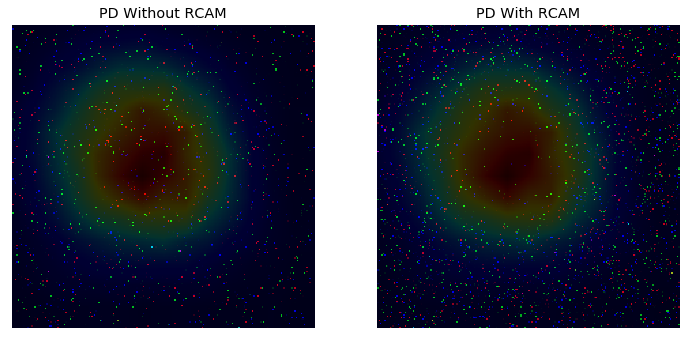
We can see that in the image which uses Pixel Deflection without RCAM the number of pixels deflected in the HOT zone (red color) is much less compared to the image that uses Pixel Deflection without RCAM.
Wavelet Denoising after PD with RCAM
img_deflected_rcam_denoised = denoiser(img_deflected_rcam)
_ = classify_images([img_deflected_rcam_denoised], true_label, visualize=True)
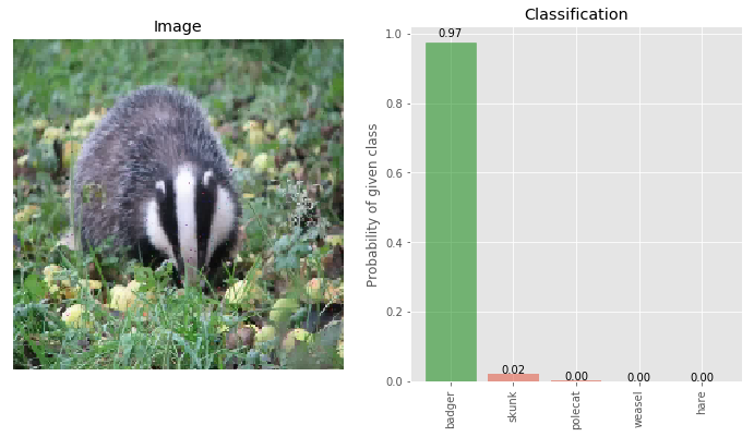
Now the confidence of the true class being badger is 97% and on the adversarial class skunk is 2%. This is our best result.
Results
| Class | Clean | Adversary | PD | PD+WD | PD+RCAM | PD+RCAM+WD |
|---|---|---|---|---|---|---|
| True class - Badger | 100 | 15 | 75 | 92 | 82 | 97 |
| Adversary - Skunk | 0.0 | 59 | 16 | 07 | 12 | 02 |
Notes
For this image, it seems a window of 20 might give better results, but for experiments, I wanted to keep the same window as reported in our paper. I have omitted the discussion of soft shrinkage for wavelet transform, which we found works much better than hard shrinkage. There is also a benefit of about 1.6% of doing YCbCr transformation from RGB before doing wavelet transform.
Strictly, this is a black-box defense as the attack model does not know the defense strategy. Randomness of the strategy makes it harder to implement a viable approximation without relying on a specific pattern of pixels. Our work is most similar to this and this.
TL;DR
Select a random pixel in the image and replace it with another pixel from the local neighbourhood. This process changes local pixel arrangement but not global statistics and thus efficiently counteracts the adversarial changes and does not impact clean images. This can be improved by selecting more pixels from regions outside of objects and by doing wavelet denoising.
For errors and corrections please contact aprakash@brandeis.edu